From the signal detection illustration, we learned that we have four possible outcomes from a signal detection situation. Below, the table describing these situations are repeated.
| Table 1(b) Signal Detection Theory Possible Situations |
|||
|---|---|---|---|
| The Signal is: | |||
| Present | Not Present | ||
| You Decide That the Signal: |
Happened | Hit | False alarm |
| Did not Happen |
Miss | Correct rejection | |
From this illustration, we learned that we can describe what is going on inside of us during a Signal Detection situation using the following figure:
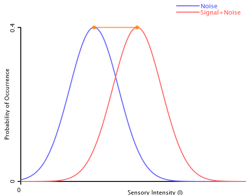
The Noise curve tells us how likely we are to have different sensory intensities for when there is not a stimulus. The Signal+Noise curve tells us how likely we are to have different sensory intensities when there is a stimulus, the signal. But how do we get from this graph to our four outcomes from a signal detection experiment?
We have left off one element. That is the criterion. You, as the observer, select a value of sensory intensity that will serve as a threshold or cutoff value. If the sensory intensity gets above that value, you will say that the signal has occurred. If the sensory intensity is below that value, then you will report that the signal has not occurred. Look at the illustration to see how the idea of the criterion can get you from this figure to the four outcomes of a signal detection situation.
To see the illustration in full screen, which is recommended, press the Full Screen button, which appears at the top of the page.
Below is a list of the ways that you can alter the model. The settings include the following:
Hits: check to display the region of the graph that generates hits. This is the area above the
criterion and under the Signal+Noise curve. The proportion of the Signal+Noise curve highlighted by the red color
give the proportion of trials that have signal that are hits.
Misses: check to display the region of the graph that generates misses. This is the area below the
criterion and under the Signal+Noise curve. The proportion of the Signal+Noise curve highlighted by the cyan color
give the proportion of trials that have signal that are misses. Hits+misses = 1.0
False Alarms: check to display the region of the graph that generates false alarms. This is the area above the
criterion and under the Noise curve. The proportion of the Noise curve highlighted by the yellowish color
give the proportion of trials that do not have a signal that are false alarms.
Correct Rejections: check to display the region of the graph that generates correct rejections. This is the area below the
criterion and under the Noise curve. The proportion of the Noise curve highlighted by the blue color
gives the proportion of trials that do not have the signal that are correct rejections. False alarms+correct rejections = 1.0
Sensitivity-d': the difference in the position of the Noise and Signal+Noise curve relates to how
easy it is to detect that the signal is present. The greater the difference, the easier the detection. We call this
difference sensitivity and measure it with the measure called d' (pronounced d-prime).
See how changing d' alters your hits and false alarm rates.
Criterion: the vertical yellow line on the pale blue line on the graph is the criterion.
You can adjust it with this slider. Lower values are more lax criterions, and higher values are more strict criterions.
Adjust to see how criterion alters hits and false alarm rates without changing d'.
Show Overlap: click to highlight the region where the Noise and Signal+Noise curves overlap. Where there is
overlap, a given stimulus intensity could be by either the noise alone or by the signal. You cannot know for certain. As you
increase d', the overlap gets smaller.
Show d': click to add a visual representation of d'. An orange line will connect the two peaks.
The larger the d', the longer the line.
Pressing this button restores the settings to their default values.